

The same shift data can give an OEE of 63.38 %, 67.60 % or 72.09 %. The shift is illustrative, and only the measurement rules change between the three figures, so each plant has to write its rules down. This guide covers the formula, two worked examples, the mistakes that move the result, and what machine data can and cannot supply. It is written for manufacturing managers, production engineers and teams moving OEE from manual spreadsheets to automated monitoring.
How to Calculate OEE: The Short Answer
Here is how to calculate OEE: OEE = Availability × Performance × Quality. When all units share one ideal cycle time, this equals good count × ideal cycle time ÷ planned production time: the share of planned production time the good units would need at that speed. Which stops count as planned is a plant rule.
What OEE Measures: The Time Model Behind the OEE Formula
OEE comes from Total Productive Maintenance (TPM) as developed in Japan by JIPM (the Japan Institute of Plant Maintenance), and Seiichi Nakajima’s Introduction to TPM (English edition 1988) made it widely known. Remove planned stops from total time to get planned production time (loading time). Remove downtime losses to get run time (operating time). Remove speed losses to get net operating time – the time the actual output would have taken at the ideal cycle time. Remove defect losses to get valuable operating time, the ideal time represented by good units. With a common ideal cycle time, availability, performance and quality are the ratios between consecutive steps of this cascade, and OEE is valuable operating time ÷ planned production time.
The cascade follows the TPM time model (Nakajima, Muchiri & Pintelon, JIPM). Which stops count as planned is a measurement rule, here this article’s declared convention. ISO 22400-2:2014 uses comparable but not identical elements (planned busy time, actual production time).
ISO 22400-2:2014 calls the comparable base planned busy time (planned operation time minus planned downtime). ISO’s name for the middle factor is effectiveness, and JIPM’s English site calls the whole metric overall equipment efficiency. The elements are comparable, not identical. ISO’s actual production time “includes only the value-adding functions”. ISO lists setup and delay separately, and the example mapping in OPC 40001-1, the OPC UA specification for machinery, allocates value-adding work performed during setup to actual production time.
Availability: How Downtime Reduces Run Time
Availability is the share of planned production time remaining after stops classified as downtime losses.
Availability = Run time ÷ Planned production time
Every stop classified as a downtime loss inside planned production time lowers availability. Two of the six big losses described in Nakajima’s book lower availability: equipment failure, and setup and adjustment. A changeover is scheduled, but in the TPM sources cited here it is not planned downtime: Nakajima’s own example counts setup minutes as stoppage losses inside loading time.
Performance: How Slow Cycles and Minor Stops Reduce Output
Performance compares what the machine produced during run time with what it would have produced at its ideal cycle time. The ideal cycle time is the time per unit that defines 100 % performance.
Performance = (Ideal cycle time × Total count) ÷ Run time = Net operating time ÷ Run time
Every minor stop or slow cycle counted inside run time lowers it. Nakajima’s speed losses sit here: idling and minor stoppages, and reduced speed. In Jonsson and Lesshammar’s (1999) rendering of Nakajima, the ideal speed is “based on the equipment capacity as initially designed”. ISO 22400-2:2014 uses a planned run time per item, “the planned time for producing one quantity unit”, and JIPM’s chart uses a standard cycle time. Which reference applies is a measurement rule (see mistake 2).
Quality: How Rejects Reduce Good Output
Quality is the share of good units in everything the machine produced.
Quality = Good count ÷ Total count
Nakajima’s defect losses lower quality: process defects, including “quality defects to be repaired”, and reduced yield from machine start-up to stable production. ISO’s quality ratio is good quantity ÷ produced quantity. Kang et al. (2016) note that this ratio in ISO 22400-2:2014 “does not include the reworked parts”. Their own model counts reworked parts as good, so rework is a rule to declare.
The Measurement Rules This Article Uses
The three-factor structure is shared. The counting rules are not. As Jonsson and Lesshammar wrote in 1999, “The exact definition of OEE differs between applications and authors.” This article applies one convention to every number:
- Planned stops (breaks, planned maintenance, scheduled meetings) are removed before planned production time.
- Changeovers and setup are downtime losses.
- Waits for material inside planned production time are downtime losses, although they are not the machine’s fault.
- Minor stops and reduced speed are speed losses.
- Rejects, including start-up rejects and units needing rework, are not good.
Other conventions count differently. ISO 22400-2:2014’s element definitions group minor stoppages with delay time. JIPM’s current chart places start-up loss under stop losses. A plant TPM profile hosted by JIPM counts preventive maintenance and changeovers inside its OEE base. TEEP, a related metric, includes planned downtime by design.
OEE Calculation Example: One Filling Machine, One 8-Hour Shift
Consider a filling machine on one 8-hour shift. The numbers are illustrative, chosen to show the arithmetic, not typical values or a benchmark.
A 480-minute shift with a planned 30-minute meal break leaves 450 minutes of planned production time. Three stops interrupt it: a capper jam (22 minutes), a changeover to a different bottle size (28 minutes) and a wait for caps (10 minutes, a downtime loss under this convention). The ideal cycle time is 1.0 second per bottle (60 bottles per minute). The machine fills 18,720 bottles: 18,252 good and 468 rejects. Minor stops were not logged as events in this example, so they sit inside the speed loss.
| Step | Calculation | Result |
|---|---|---|
| 1. Planned production time | 480 min – 30 min | 450 min |
| 2. Run time | 450 min – (22 + 28 + 10) min | 390 min |
| 3. Availability | 390 ÷ 450 | 86.67 % |
| 4. Net operating time | 18,720 × 1.0 s = 18,720 s | 312 min |
| 5. Performance | 312 ÷ 390 | 80.00 % |
| 6. Quality | 18,252 ÷ 18,720 | 97.50 % |
| 7. OEE | 86.67 % × 80.00 % × 97.50 % | 67.60 % |
| 8. Cross-check | 18,252 × 1.0 s ÷ (450 × 60 s) = 18,252 ÷ 27,000 | 67.60 % |
Percentages in the tables are calculated from unrounded figures and displayed to two decimals. In minutes, the losses split like this:
| Loss | Minutes | Share of planned production time | Where it comes from |
|---|---|---|---|
| Downtime losses (availability) | 60.0 | 13.33 % | three logged events: changeover 28, jam 22, caps 10 |
| Speed losses (performance) | 78.0 | 17.33 % | 390 run minutes produced only 312 minutes’ worth of bottles at the ideal rate · not tied to any logged event |
| Defect losses (quality) | 7.8 | 1.73 % | 468 rejected bottles × 1.0 s |
| Valuable operating time | 304.2 | 67.60 % | – |
| Total | 450.0 | 100.00 % | check closes |
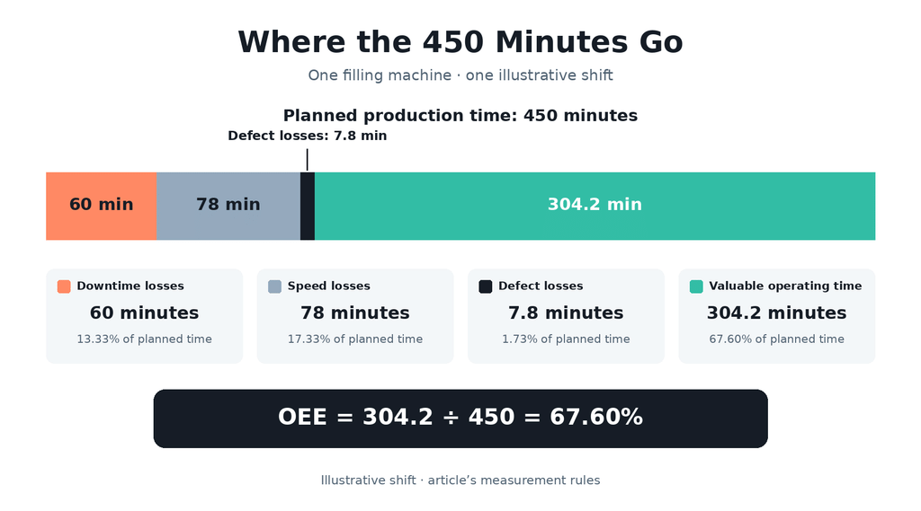
Which losses deserve attention? These numbers alone show three things:
- Speed losses are the largest bucket (78 minutes) and the only one with no logged cause. Before acting, an engineer should find out whether those minutes are short stops, slow running or a wrong ideal cycle time.
- The 28-minute changeover is the largest logged event, yet it is smaller than the unexplained speed loss.
- Defect losses are the smallest in time (7.8 minutes). That does not make them the smallest in cost: Bengtsson et al. (2020) point out that OEE applies “no weighting among availability, performance, and quality”.
OEE for Multiple Machines: State the Objective, Then Combine
The cited sources do not prescribe a single plant OEE. If the plant figure should show what share of all scheduled machine time produced good output at ideal speed, add up the times first, then divide.
Now add a case packer, machine B, with one scheduled 150-minute run. It loses 40 minutes to a changeover and 20 minutes to a jam, has an ideal cycle time of 2.0 seconds and processes 2,250 units, 2,160 of them good.
| Machine | Planned production time | Run time | Ideal cycle time | Total | Good | A | P | Q | OEE | Valuable operating time |
|---|---|---|---|---|---|---|---|---|---|---|
| A – filler (the worked-example machine) | 450 min | 390 min | 1.0 s | 18,720 | 18,252 | 86.67 % | 80.00 % | 97.50 % | 67.60 % | 304.2 min |
| B – case packer | 150 min (one scheduled run) | 90 min (40-min changeover + 20-min jam) | 2.0 s | 2,250 | 2,160 | 60.00 % | 83.33 % | 96.00 % | 48.00 % | 72.0 min |
| Simple average of the two percentages | – | – | – | – | – | – | – | – | 57.80 % (wrong for this objective) | – |
| Summed times | 600 machine-minutes | – | – | – | – | – | – | – | 62.70 % = 376.2 ÷ 600 | 376.2 min |
The simple average (57.80 %) gives the 150-minute run the same weight as the 450-minute shift. Summing valuable operating time and dividing by summed planned production time gives 376.2 ÷ 600 = 62.70 %, which equals the average weighted by planned production time. Here the simple average understates by 4.9 points, and had the shorter run scored higher, it would have overstated. Adding the two good counts and multiplying by the filler’s 1.0-second cycle time is also wrong when cycle times differ: it gives 56.70 %.
Equal machine weights are a legitimate, different metric when declared. Moradizadeh and Mayorga (2014) call it “overall line efficiency”. A serial line (filler → capper → labeller) needs a line model for losses from bottlenecks and synchronisation (Braglia et al., Teoh et al.), not an average, product or minimum of station OEEs.
Common OEE Calculation Mistakes
- Inconsistent time definitions. Counting the meal break inside the base drops availability from 86.67 % to 81.25 % and OEE from 67.60 % to 63.38 %, while reclassifying the 28-minute changeover as planned lifts OEE to 72.09 %. Hedman et al. (2016), citing earlier research, call the interpretation of the loss factors “a common reason for variations between companies”.
- A wrong ideal cycle time. A slower reference inflates performance, and a faster one depresses it. With 1.3 seconds instead of 1.0, performance reads 104 % and OEE 87.88 %. With 0.9 seconds, they read 72 % and 60.84 %. Bengtsson et al. (2020) note that with increased cycle times “the OEE-value might increase while the actual productivity might decrease”. Warning sign: performance above 100 % is a signal to check the ideal cycle time, units, counters and time windows.
- Averaging percentages without a weighting rule. Short runs then weigh as much as long ones, which gives 57.80 % instead of 62.70 % in the two-machine example.
- Counting the same loss twice. Using good count in performance and then multiplying by quality penalises the same rejects twice (65.91 % instead of 67.60 %). Subtracting 5 minutes of minor stops from run time while leaving performance at 80.00 % lowers OEE to 66.73 %. If performance is recalculated from total count and the shorter run time, OEE stays at 67.60 %.
- Counting reworked units as good without declaring it. If 300 of the 468 rejects were reworked and counted as good, quality would read 99.10 % and OEE 68.71 %.
- Leaving performance and quality at default values. OEE then collapses into availability. In a study of 23 Swedish companies, 884 machines and one automatic OEE system (2013–14), Hedman et al. (2016) found performance recorded as 100 % on 702 machines and quality on 796, where 100 % was the system’s default. In their words, “it can be questioned if companies really are measuring the overall equipment efficiency or just the availability.”
- No written minor-stop rule, and downtime logged as “other”. Minor stops then land in availability on one line and in performance on another. In the same study, unclassified losses were “about 19% of the scheduled production time”. The cited specifications do not set a numerical minor-stop threshold. The example mapping in OPC 40001-1 says “time is just out of cycle time”.
- Comparing OEE across unlike machines or plants, or grading it against 85 %. Bengtsson et al. (2020) write that OEE “is generally not a good indicator for comparison between companies or even machines”. Comparisons of the same machine over time also need to account for changes in production articles and ideal cycle time. The next section explains where 85 % comes from.
How to Interpret an OEE Result
Rule of thumb: a result of 67.60 % is neither good nor bad on its own – it gains meaning when compared with the same machine, under the same rules, over time. Beyond the measurement rules, three kinds of context matter.
Equipment type: JIPM notes that process industries define the three factors differently, and ISO 22400-2:2014 says KPIs from its production order time model “need to be adjusted” for continuous processes.
Product mix: when one machine runs several products, performance has to sum ideal time × count per product, as the worked example in ISO/TR 22400-10 does. Bengtsson et al. liken comparing machines with different product-mix profiles to “comparing apples with oranges”.
Surroundings: writing about semiconductor equipment, de Ron and Rooda (2005) note that OEE “does include equipment-independent conditions, such as lack of input items”, which are “not caused by the equipment”.
Where does 85 % come from? Nakajima’s Introduction to TPM (English edition 1988) describes an OEE of about 85 % (availability greater than 90 %, performance greater than 95 %, quality greater than 99 %) as ideal conditions, “based on our experience”. The same book warns that companies’ methods of calculation “vary widely”.
The cited evidence does not establish a transferable industry benchmark for whether 67.60 % is good for this machine, or how much replacing operator logs with automatic capture would change its OEE. ISO has also marked ISO 22400-2:2014 itself for revision.
OEE from PLC Data: What Machines Provide and What People Decide
PLC data, production counters and downtime records give machine states, durations and counts. Planned busy time and the planned run time per item “usually” come from an MES or ERP “and not from the machine”, according to an informative annex of OPC 40501-1, an OPC UA machine-tool companion specification. PackML is a common model of machine states and tags (technical report ISA-TR88.00.02). Tag names below follow the OPC Foundation’s PackML model (OPC 30050), and all PackML Admin tags are optional.
| OEE input | Data source on the machine | Spec reference |
|---|---|---|
| Planned production time (comparable ISO element: planned busy time) | Usually supplied by an operation calendar or production schedule in an MES or ERP, according to the cited machine-tool model. | OPC 40501-1 Annex C.2.4: “This information usually comes from an MES or ERP and not from the machine” · OPC 40001-1 Annex C.2: system state “based on operation calendar” |
| Run time and downtime | Machine states timed by the client, or PackML StateCumulativeTime counters: OPC UA Machinery states with operation mode, PackML Execute / Held / Suspended / Stopped, MTConnect Execution (ACTIVE, STOPPED, INTERRUPTED …) | OPC 40001-1 §12, Annex C.2 Table 68 (“proposes” a mapping) · OPC 30050 §6.3.4 StateCumulativeTime · OPC 40501-1 C.2.2: “the status duration must be measured” |
| Planned vs unplanned, setup vs maintenance | Not decided by the state signal. Operation mode “may not be known by the MachineryItem itself” → MES or operator | OPC 40001-1 §13.1 |
| Downtime reason | PackML StopReason records the first event captured during an abort, held, suspended or stop event. First-out fault reporting is a typical use, and the event still needs a declared OEE loss-category mapping. | OPC 30050 §6.3.4 |
| Blocked / starved | PackML Suspended: “conditions external to the unit/machine require a pause in production” | OPC 30050 §6.3.8 |
| Total count | PackML ProdProcessedCount · OPC UA PartsProducedInLifetime (difference over the order) or job PartsCompleted · MTConnect PartCount ALL | OPC 30050 §6.3.4 · OPC 40501-1 C.2.1 · MTConnect Part 3 v2.5.0 |
| Good count | PackML processed minus ProdDefectiveCount (“the number of non-defective products made by the machine”) · job PartsGood · MTConnect PartCount GOOD – when a suitable quality source is available. GQ “cannot be determined via the PartsProducedInLifetime” | OPC 30050 §6.3.4 · OPC 40501-1 C.2.1 · NIST/Boeing 2016: quality often decided later in the process |
| Rework | Usually none: “The machine does not usually provide a count of rework” | OPC 40501-1 C.2.1 |
| Ideal cycle time | Planned run time per item “usually comes from an MES or ERP”. PackML MachDesignSpeed is a candidate, defined for the installed environment and package configuration, “NOT the maximum speed as specified by the manufacturer” | OPC 40501-1 C.2.4 · OPC 30050 §6.3.4 |
| Speed loss | State signals alone do not quantify speed loss. The cited mapping says technological effects such as waits for feeds or drains require analysis on SCADA or machinery level. PackML CurMachSpeed reports current speed. | OPC 40001-1 Annex C.2 Note 2 · OPC 30050 §6.3.3 |
| Counter period | PackML AccCount: “a non-resetting counter that may be used for OEE calculations” · MTConnect resetTriggered (e.g. SHIFT) · OPC lifetime counters never reset | OPC 30050 §6.5.3 · MTConnect Part 3 · OPC 40001-1 §14.2 |
| Terminology trap | MTConnect “Availability” means the “agent’s ability to communicate with the data source”, not OEE availability | MTConnect Part 3 v2.5.0 |
Automated collection can record the configured machine states, counts and timestamps. Coverage depends on the available signals and the capture configuration. Automation does not decide:
- the planned-time calendar
- which machine state counts as which loss
- the minor-stop rule and the reason-code categories
- the stored ideal cycle time for each item
- where quality and rework counts come from
- when counters reset
- who is charged for blocked or starved time
- what happens to default values
People make those decisions, so automation supports consistent calculation once the rules are written down.
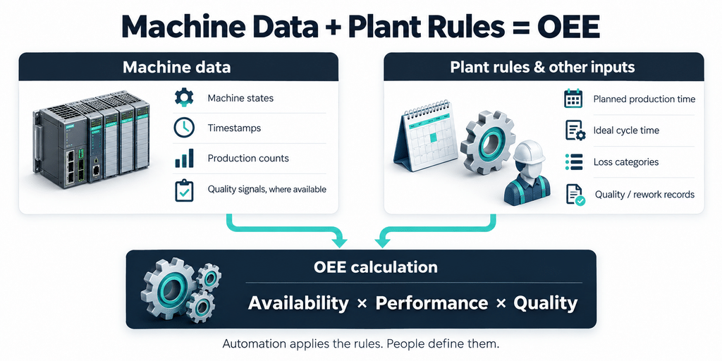
Hedman et al. (2016) conclude that how well the measures reflect what the equipment does “is directly dependent on how well companies are able to interpret and define the underlying factors of OEE”. Their study covered 23 Swedish companies, 884 machines and one automatic OEE system in 2013–14. The same authors add that the technical system “indeed has the capability” to handle these issues once companies define the core data.
Readers comparing tools that collect this data can start with the overview of real-time machine monitoring platforms.
Iotellect is one platform for building production dashboards on this data. Its SCADA software connects to PLCs and field devices over protocols including OPC UA, OPC DA/HDA/AE, Modbus, Siemens S7 and Omron FINS, reading data in real time. The Iotellect MES reads directly from the same tag database the SCADA uses. It calculates OEE automatically from real-time machine data, with availability, performance and quality broken down per line, shift, or product, and tracks every downtime event with reason codes. Behind Iotellect’s OEE tracking in an MES, the OEE calculations, like the scheduling logic and the workflow rules, are visible and editable through a visual interface. Role-based dashboards show work order progress, cycle times, output counts and quality rates to operators, supervisors and plant management. The plant team or its integrator decides the rules (planned time, ideal cycle times, reason codes). Iotellect supplies the platform.
Frequently Asked Questions
How do you calculate OEE?
Multiply availability, performance and quality. Availability is run time ÷ planned production time, performance is ideal cycle time × total count ÷ run time, and quality is good count ÷ total count. With a common ideal cycle time, a single division gives the same result: good count × ideal cycle time ÷ planned production time. The plant decides which stops are planned.
What is an example of an OEE calculation?
In the illustrative filling-machine shift above, availability is 86.67 %, performance 80.00 % and quality 97.50 %, so OEE is 67.60 %. The cross-check, 18,252 good bottles × 1.0 second ÷ 27,000 seconds of planned production time, gives the same 67.60 %.
What is the difference between OEE and availability?
Availability is one of the three OEE factors and reflects stops classified as downtime, while OEE also counts speed and quality losses. With a correctly set ideal cycle time, OEE cannot exceed availability: in the example, availability is 86.67 % and OEE is 67.60 %. A related metric, TEEP, includes planned downtime by using calendar time (Muchiri and Pintelon 2008, Iannone and Nenni 2013).
Is planned downtime included in OEE?
It depends on the convention. Nakajima’s example removes scheduled maintenance and morning meetings before loading time (planned production time), and ISO 22400-2:2014’s planned busy time subtracts planned downtime. Muchiri and Pintelon (2008) recommend that scheduled downtime “should therefore not be used in OEE calculation”, while TEEP includes it by design. A plant may also define it in. Changeovers are downtime losses under this article’s convention and in Nakajima’s example, even when scheduled. Write the rule down.
How do you calculate OEE for multiple machines?
The cited sources do not prescribe a single plant OEE. If the plant figure should show how much scheduled time on all machines went into good output at ideal speed, divide summed valuable operating time by summed planned production time. That equals an average weighted by planned production time: 62.70 % in the example, against 57.80 % for the simple average. A serial line needs its own line model.
Can OEE be calculated automatically from PLC data?
Partly. Machine states and counts can be read automatically, and durations can be measured from states. In the cited machine-tool model, planned time and the planned run time per item usually come from an MES or ERP, and rework is usually not supplied. Quality may need job data or operator input.